Getting Started
The purpose of the present Getting Started section is to give a quick overview of the main objects and features of the LArray library. To get a more detailed presentation of all capabilities of LArray, read the next sections of the tutorial. The API Reference section of the documentation give you the list of all objects, methods and functions with their individual documentation and examples.
To use the LArray library, the first thing to do is to import it:
In [1]: from larray import *
Create an array
Working with the LArray library mainly consists of manipulating LArray data structures. They represent N-dimensional labelled arrays and are composed of raw data (NumPy ndarray), axes and optionally some metadata.
An axis represents a dimension of an array. It contains a list of labels and has a name:
# define some axes to be used later
In [2]: age = Axis(['0-9', '10-17', '18-66', '67+'], 'age')

In [3]: sex = Axis(['F', 'M'], 'sex')

In [4]: year = Axis([2015, 2016, 2017], 'year')
The labels allow to select subsets and to manipulate the data without working with the positions of array elements directly.
To create an array from scratch, you need to supply data and axes:
# define some data. This is the belgian population (in thousands). Source: eurostat.
In [5]: data = [[[633, 635, 634],
   ...:          [663, 665, 664]],
   ...:         [[484, 486, 491],
   ...:          [505, 511, 516]],
   ...:         [[3572, 3581, 3583],
   ...:          [3600, 3618, 3616]],
   ...:         [[1023, 1038, 1053],
   ...:          [756, 775, 793]]]
   ...:

# create an LArray object
In [6]: pop = LArray(data, axes=[age, sex, year])

In [7]: pop
Out[7]:
  age  sex\year  2015  2016  2017
  0-9         F   633   635   634
  0-9         M   663   665   664
10-17         F   484   486   491
10-17         M   505   511   516
18-66         F  3572  3581  3583
18-66         M  3600  3618  3616
  67+         F  1023  1038  1053
  67+         M   756   775   793
You can optionally attach some metadata to an array:
# attach some metadata to the pop array
In [8]: pop.meta.title = 'population by age, sex and year'

In [9]: pop.meta.source = 'Eurostat'

# display metadata
In [10]: pop.meta
Out[10]:
title: population by age, sex and year
source: Eurostat
To get a short summary of an array, type:
# Array summary: metadata + dimensions + description of axes
In [11]: pop.info
Out[11]:
title: population by age, sex and year
source: Eurostat
4 x 2 x 3
 age [4]: '0-9' '10-17' '18-66' '67+'
 sex [2]: 'F' 'M'
 year [3]: 2015 2016 2017
dtype: int64
memory used: 192 bytes
Create an array filled with predefined values
Arrays filled with predefined values can be generated through dedicated functions:
zeros(): creates an array filled with 0
In [12]: zeros([age, sex])
Out[12]:
age\sex    F    M
    0-9  0.0  0.0
  10-17  0.0  0.0
  18-66  0.0  0.0
    67+  0.0  0.0
ones(): creates an array filled with 1
In [13]: ones([age, sex])
Out[13]:
age\sex    F    M
    0-9  1.0  1.0
  10-17  1.0  1.0
  18-66  1.0  1.0
    67+  1.0  1.0
full(): creates an array filled with a given value
In [14]: full([age, sex], fill_value=10.0)
Out[14]:
age\sex     F     M
    0-9  10.0  10.0
  10-17  10.0  10.0
  18-66  10.0  10.0
    67+  10.0  10.0
sequence(): creates an array by sequentially applying modifications to the array along axis.
In [15]: sequence(age)
Out[15]:
age  0-9  10-17  18-66  67+
       0      1      2    3
ndtest(): creates a test array with increasing numbers as data
In [16]: ndtest([age, sex])
Out[16]:
age\sex  F  M
    0-9  0  1
  10-17  2  3
  18-66  4  5
    67+  6  7
Save/Load an array
The LArray library offers many I/O functions to read and write arrays in various formats
(CSV, Excel, HDF5). For example, to save an array in a CSV file, call the method
to_csv():
# save our pop array to a CSV file
In [17]: pop.to_csv('belgium_pop.csv')
The content of the CSV file is then:
age,sex\time,2015,2016,2017
0-9,F,633,635,634
0-9,M,663,665,664
10-17,F,484,486,491
10-17,M,505,511,516
18-66,F,3572,3581,3583
18-66,M,3600,3618,3616
67+,F,1023,1038,1053
67+,M,756,775,793
Note
In CSV or Excel files, the last dimension is horizontal and the names of the
last two dimensions are separated by a \.
To load a saved array, call the function read_csv():
In [18]: pop = read_csv('belgium_pop.csv')

In [19]: pop
Out[19]:
  age  sex\year  2015  2016  2017
  0-9         F   633   635   634
  0-9         M   663   665   664
10-17         F   484   486   491
10-17         M   505   511   516
18-66         F  3572  3581  3583
18-66         M  3600  3618  3616
  67+         F  1023  1038  1053
  67+         M   756   775   793
Other input/output functions are described in the Input/Output section of the API documentation.
Selecting a subset
To select an element or a subset of an array, use brackets [ ]. In Python we usually use the term indexing for this operation.
Let us start by selecting a single element:
In [20]: pop['67+', 'F', 2017]
Out[20]: 1053
Labels can be given in arbitrary order:
In [21]: pop[2017, 'F', '67+']
Out[21]: 1053
When selecting a larger subset the result is an array:
In [22]: pop[2017]
Out[22]:
age\sex F M
0-9 634 664
10-17 491 516
18-66 3583 3616
67+ 1053 793
In [23]: pop['M']
��������������������������������������������������������������������������������������������������������������Out[23]:
age\year 2015 2016 2017
0-9 663 665 664
10-17 505 511 516
18-66 3600 3618 3616
67+ 756 775 793
When selecting several labels for the same axis, they must be given as a list (enclosed by [ ])
In [24]: pop['F', ['0-9', '10-17']]
Out[24]:
age\year  2015  2016  2017
     0-9   633   635   634
   10-17   484   486   491
You can also select slices, which are all labels between two bounds (we usually call them the start and stop bounds). Specifying the start and stop bounds of a slice is optional: when not given, start is the first label of the corresponding axis, stop the last one:
# in this case '10-17':'67+' is equivalent to ['10-17', '18-66', '67+']
In [25]: pop['F', '10-17':'67+']
Out[25]:
age\year 2015 2016 2017
10-17 484 486 491
18-66 3572 3581 3583
67+ 1023 1038 1053
# :'18-66' selects all labels between the first one and '18-66'
# 2017: selects all labels between 2017 and the last one
In [26]: pop[:'18-66', 2017:]
����������������������������������������������������������������������������������������������������������������������Out[26]:
age sex\year 2017
0-9 F 634
0-9 M 664
10-17 F 491
10-17 M 516
18-66 F 3583
18-66 M 3616
Note
Contrary to slices on normal Python lists, the stop bound is included in the selection.
Warning
Selecting by labels as above only works as long as there is no ambiguity. When several axes have some labels in common and you do not specify explicitly on which axis to work, it fails with an error ending with something like ValueError: <somelabel> is ambiguous (valid in <axis1>, <axis2>).
For example, let us create a test array with an ambiguous label. We first create an axis (some kind of status code) with an ‘F’ label (remember we already have an ‘F’ label on the sex axis).
In [27]: status = Axis(['A', 'C', 'F'], 'status')
Then create a test array using both axes ‘sex’ and ‘status’:
In [28]: ambiguous_arr = ndtest([sex, status, year])

In [29]: ambiguous_arr
Out[29]:
sex  status\year  2015  2016  2017
  F            A     0     1     2
  F            C     3     4     5
  F            F     6     7     8
  M            A     9    10    11
  M            C    12    13    14
  M            F    15    16    17
If we try to get the subset of our array concerning women (represented by the ‘F’ label in our array), we might try something like:
In [30]: ambiguous_arr[2017, 'F']
… but we receive back a volley of insults
[some long error message ending with the line below]
[...]
ValueError: F is ambiguous (valid in sex, status)
In that case, we have to specify explicitly which axis the ‘F’ label we want to select belongs to:
In [31]: ambiguous_arr[2017, sex['F']]
Out[31]:
status  A  C  F
        2  5  8
Aggregation
The LArray library includes many aggregations methods: sum, mean, min, max, std, var, …
For example, assuming we still have an array in the pop variable:
In [32]: pop
Out[32]:
  age  sex\year  2015  2016  2017
  0-9         F   633   635   634
  0-9         M   663   665   664
10-17         F   484   486   491
10-17         M   505   511   516
18-66         F  3572  3581  3583
18-66         M  3600  3618  3616
  67+         F  1023  1038  1053
  67+         M   756   775   793
We can sum along the ‘sex’ axis using:
In [33]: pop.sum(sex)
Out[33]:
age\year  2015  2016  2017
     0-9  1296  1300  1298
   10-17   989   997  1007
   18-66  7172  7199  7199
     67+  1779  1813  1846
Or sum along both ‘age’ and ‘sex’:
In [34]: pop.sum(age, sex)
Out[34]:
year   2015   2016   2017
      11236  11309  11350
It is sometimes more convenient to aggregate along all axes except some. In that case, use the aggregation methods ending with _by. For example:
In [35]: pop.sum_by(year)
Out[35]:
year   2015   2016   2017
      11236  11309  11350
Groups
A Group represents a subset of labels or positions of an axis:
In [36]: children = age['0-9', '10-17']

In [37]: children
Out[37]: age['0-9', '10-17']
It is often useful to attach them an explicit name using the >> operator:
In [38]: working = age['18-66'] >> 'working'

In [39]: working
Out[39]: age['18-66'] >> 'working'

In [40]: nonworking = age['0-9', '10-17', '67+'] >> 'nonworking'

In [41]: nonworking
Out[41]: age['0-9', '10-17', '67+'] >> 'nonworking'
Still using the same pop array:
In [42]: pop
Out[42]:
  age  sex\year  2015  2016  2017
  0-9         F   633   635   634
  0-9         M   663   665   664
10-17         F   484   486   491
10-17         M   505   511   516
18-66         F  3572  3581  3583
18-66         M  3600  3618  3616
  67+         F  1023  1038  1053
  67+         M   756   775   793
Groups can be used in selections:
In [43]: pop[working]
Out[43]:
sex\year 2015 2016 2017
F 3572 3581 3583
M 3600 3618 3616
In [44]: pop[nonworking]
�������������������������������������������������������������������������������������������Out[44]:
age sex\year 2015 2016 2017
0-9 F 633 635 634
0-9 M 663 665 664
10-17 F 484 486 491
10-17 M 505 511 516
67+ F 1023 1038 1053
67+ M 756 775 793
or aggregations:
In [45]: pop.sum(nonworking)
Out[45]:
sex\year  2015  2016  2017
       F  2140  2159  2178
       M  1924  1951  1973
When aggregating several groups, the names we set above using >> determines the label on the aggregated axis.
Since we did not give a name for the children group, the resulting label is generated automatically :
In [46]: pop.sum((children, working, nonworking))
Out[46]:
       age  sex\year  2015  2016  2017
 0-9,10-17         F  1117  1121  1125
 0-9,10-17         M  1168  1176  1180
   working         F  3572  3581  3583
   working         M  3600  3618  3616
nonworking         F  2140  2159  2178
nonworking         M  1924  1951  1973
Grouping arrays in a Session
Arrays may be grouped in Session objects. A session is an ordered dict-like container of LArray objects with special I/O methods. To create a session, you need to pass a list of pairs (array_name, array):
In [47]: pop = zeros([age, sex, year])
In [48]: births = zeros([age, sex, year])
In [49]: deaths = zeros([age, sex, year])
# create a session containing the three arrays 'pop', 'births' and 'deaths'
In [50]: demo = Session(pop=pop, births=births, deaths=deaths)
# displays names of arrays contained in the session
In [51]: demo.names
Out[51]: ['births', 'deaths', 'pop']
# get an array
In [52]: demo['pop']
�������������������������������������Out[52]:
age sex\year 2015 2016 2017
0-9 F 0.0 0.0 0.0
0-9 M 0.0 0.0 0.0
10-17 F 0.0 0.0 0.0
10-17 M 0.0 0.0 0.0
18-66 F 0.0 0.0 0.0
18-66 M 0.0 0.0 0.0
67+ F 0.0 0.0 0.0
67+ M 0.0 0.0 0.0
# add/modify an array
In [53]: demo['foreigners'] = zeros([age, sex, year])
Warning
If you are using a Python version prior to 3.6, you will have to pass a list of pairs to the Session constructor otherwise the arrays will be stored in an arbitrary order in the new session. For example, the session above must be created using the syntax: demo=Session([(‘pop’, pop), (‘births’, births), (‘deaths’, deaths)]).
One of the main interests of using sessions is to save and load many arrays at once:
# dump all arrays contained in the session 'demo' in one HDF5 file
In [54]: demo.save('demo.h5')

# load all arrays saved in the HDF5 file 'demo.h5' and store them in the session 'demo'
In [55]: demo = Session('demo.h5')
Graphical User Interface (viewer)
The LArray project provides an optional package called larray-editor allowing users to explore and edit arrays through a graphical interface. The larray-editor tool is automatically available when installing the larrayenv metapackage from conda.
To explore the content of arrays in read-only mode, import larray-editor and call view()
In [56]: from larray_editor import *

# shows the arrays of a given session in a graphical user interface
In [57]: view(ses)

# the session may be directly loaded from a file
In [58]: view('my_session.h5')

# creates a session with all existing arrays from the current namespace
# and shows its content
In [59]: view()
To open the user interface in edit mode, call edit() instead.
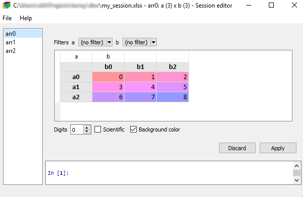
Once open, you can save and load any session using the File menu.
Finally, you can also visually compare two arrays or sessions using the compare() function.
In [60]: arr0 = ndtest((3, 3))

In [61]: arr1 = ndtest((3, 3))

In [62]: arr1[['a1', 'a2']] = -arr1[['a1', 'a2']]

In [63]: compare(arr0, arr1)
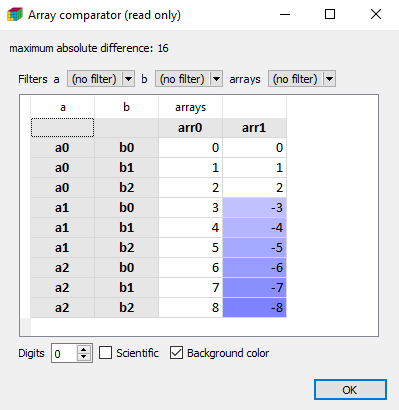
In case of two arrays, they must have compatible axes.
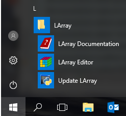
For Windows Users
Installing the larray-editor package on Windows will create a LArray menu in the
Windows Start Menu. This menu contains:
a shortcut to open the documentation of the last stable version of the library
a shortcut to open the graphical interface in edit mode.
a shortcut to update larrayenv.
Once the graphical interface is open, all LArray objects and functions are directly accessible. No need to start by from larray import *.